
PyTrendy





Welcome
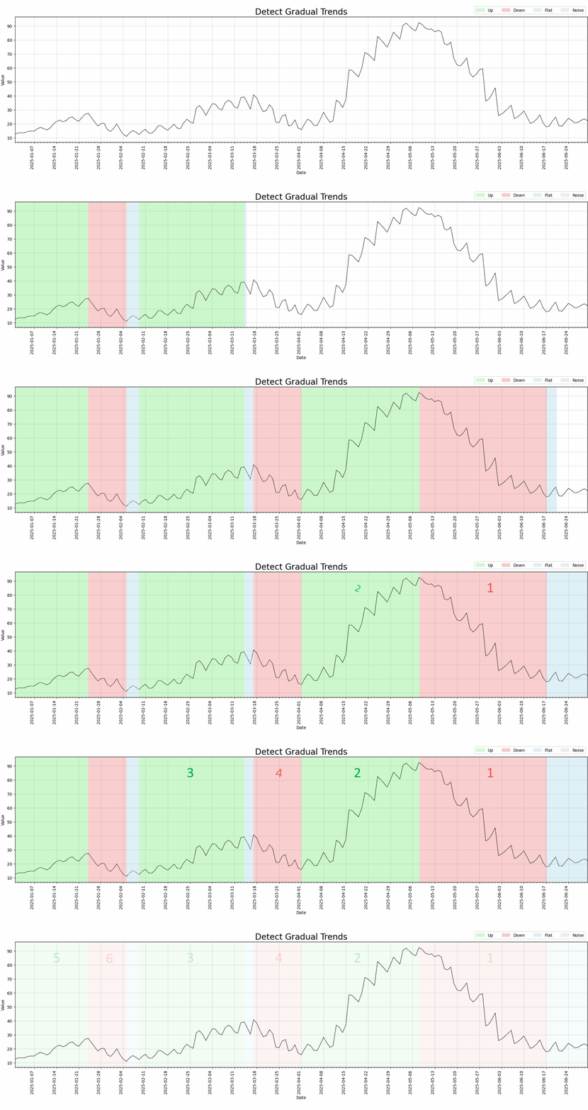
PyTrendy is a robust solution for identifying and analysing trends in time series. Unlike other packages, it detects uptrends and downtrends without falsely detecting them over flat or noisy periods.
It is a thoughtful algorithm with a focus on signal processing and post-processing, aiming to be the best package for trend detection in Python.
Why PyTrendy?
Most time series tools give you either a "trend component" (via decomposition) or "changepoints" (the moments of shift). PyTrendy is built for automated trend detection, answering what trends existed, how strong were they, and when did they start and end?
PyTrendy improves on existing methods in three ways:
- Beyond step changes -
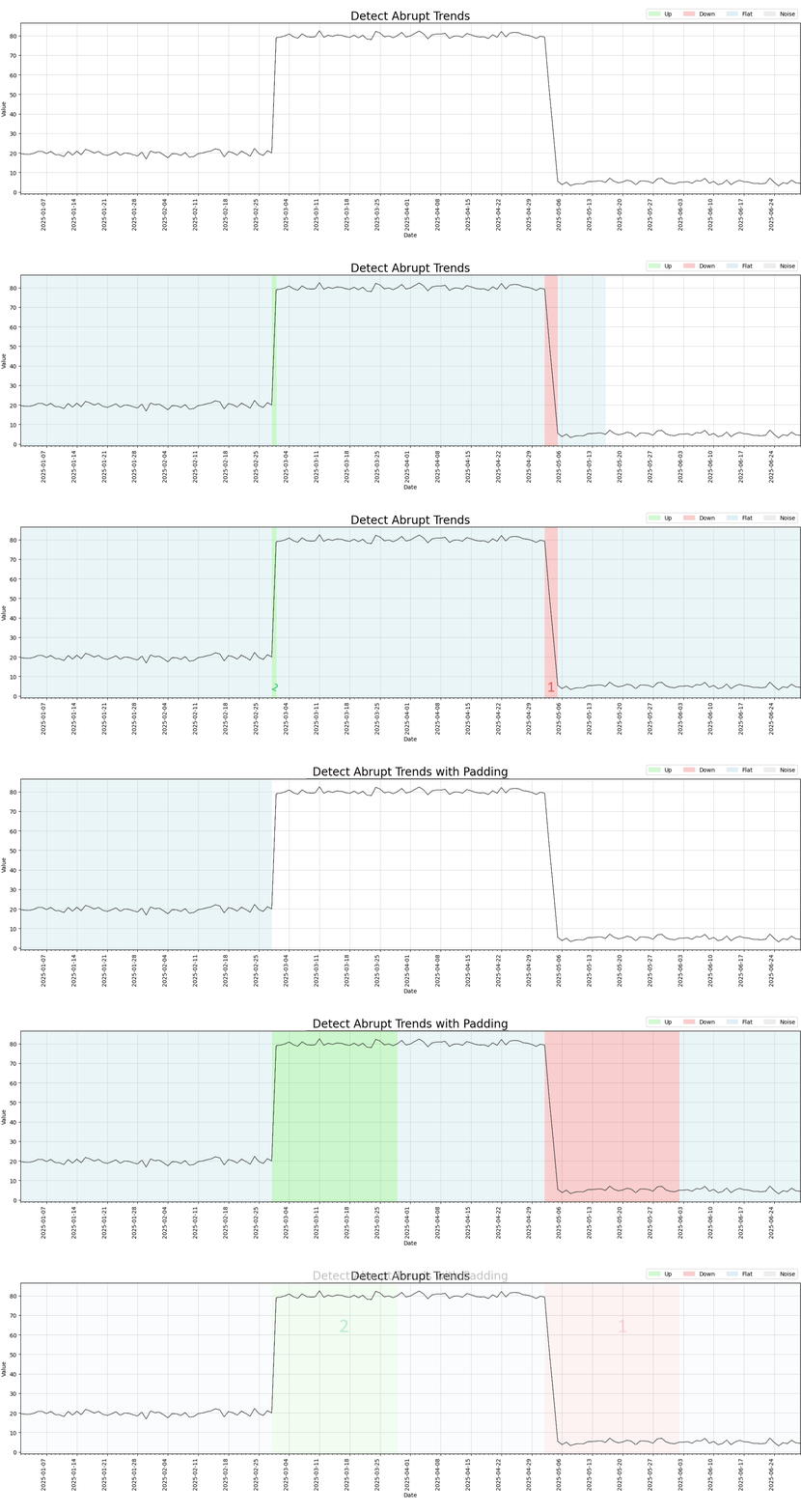
rupturesis the gold standard for abrupt shifts, but it doesn't handle gradual slope changes: the kind often seen in digital marketing activity, stock trends, and energy time series. PyTrendy detects both gradual and abrupt trends in a single run. - The flat/noise problem - the closest peers (
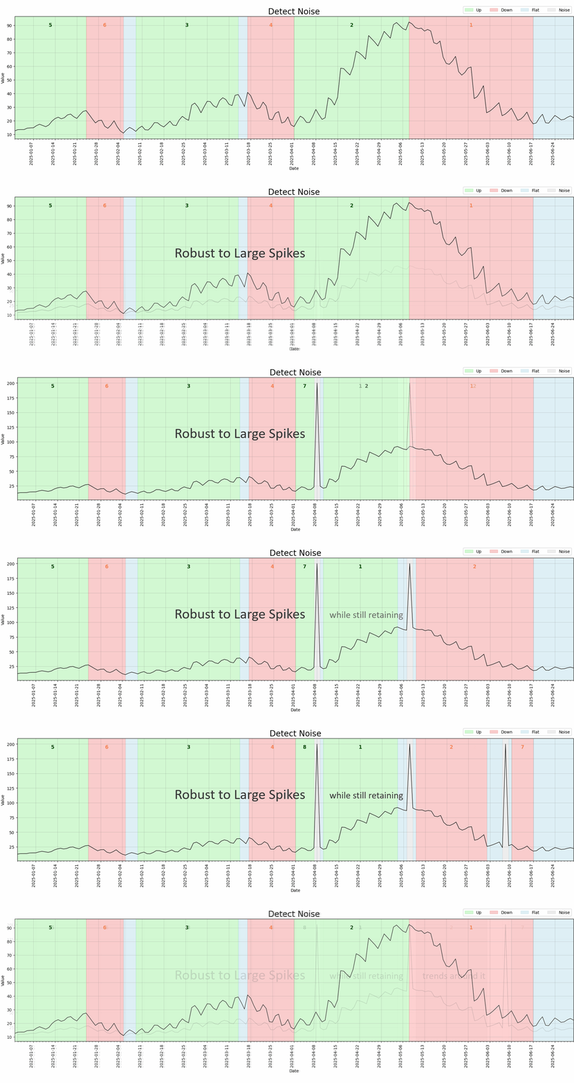
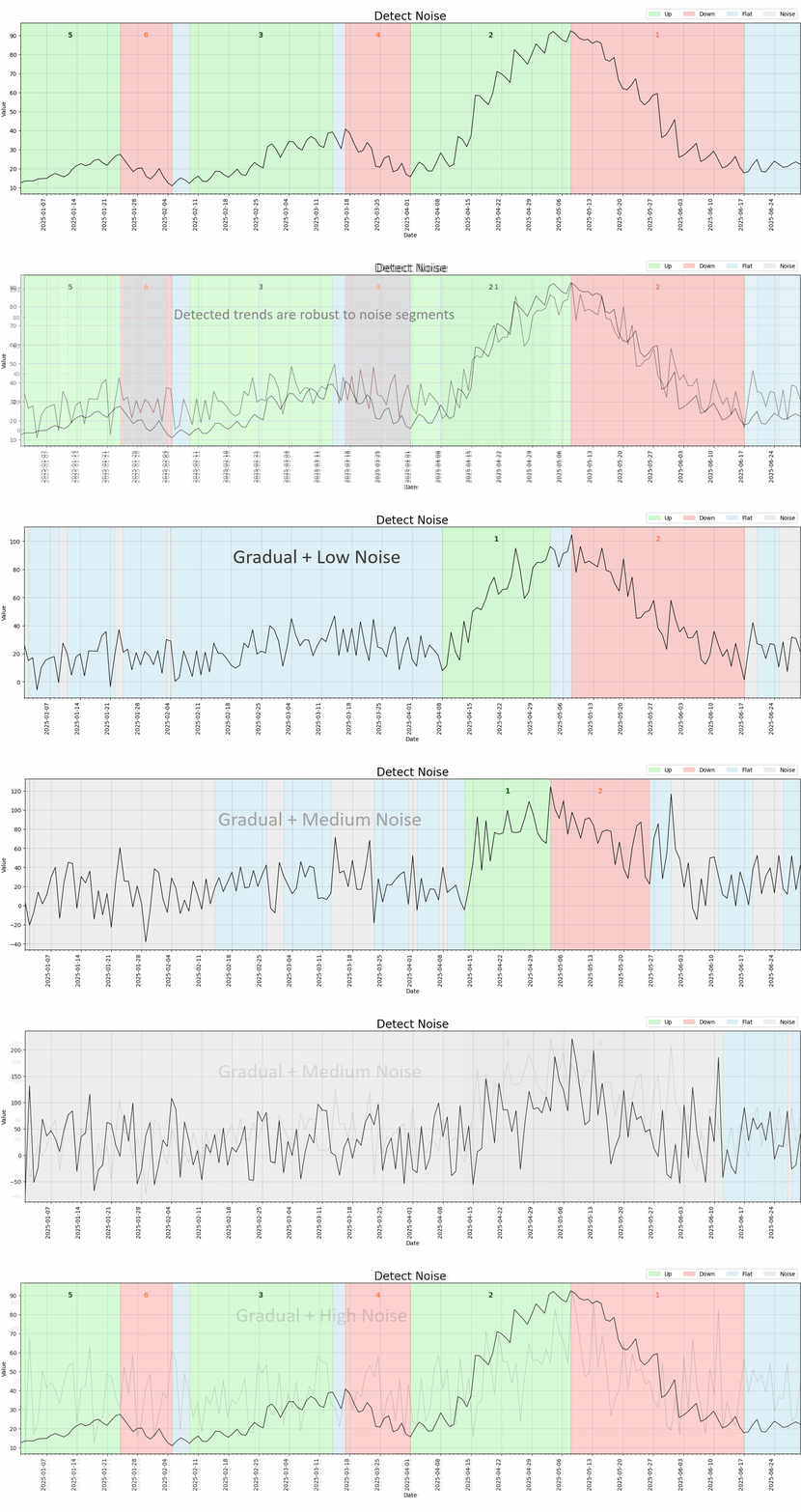
pytrendseries,trendet,tstrends) tend to over-fit trends on flat or noisy periods, leaving users to build labour-intensive workarounds. PyTrendy uses signal processing and post-processing under the hood so trends are only detected when they are precise and valid. - Strategic value - in a complex ecosystem where dozens of time series interact, knowing exactly how they align or confound each other at specific times is invaluable. Without accurately labelling the "before and after" of historical data, experiments can fly blind and generate misleading indications.
Trend detection has several use cases, such as analysing stock prices, identifying demand patterns in seasonality, and scanning Google Trends at scale for emerging movements. A main use case is identifying different periods of marketing activity at scale, to help observationally measure the effectiveness of digital marketing. By applying it to daily marketing spend (treatment), it identifies valid treatment (uptrends/downtrends) and placebo (flat) periods for observational causal inference. Applied to the response of an experiment design, it can also flag periods of noise (such as sales promotions) to mitigate the risk of misleading indications.
Features
Installation
Install the package from PyPi.
pip install pytrendy
Alternatively, if you want the latest pre-release
pip install --pre pytrendy
Quickstart
Import pytrendy, and apply trend detection on daily time series data.
import pytrendy as pt
df = pt.load_data('series_synthetic')
results = pt.detect_trends(df, date_col='date', value_col='gradual', plot=True)
results.print_summary()
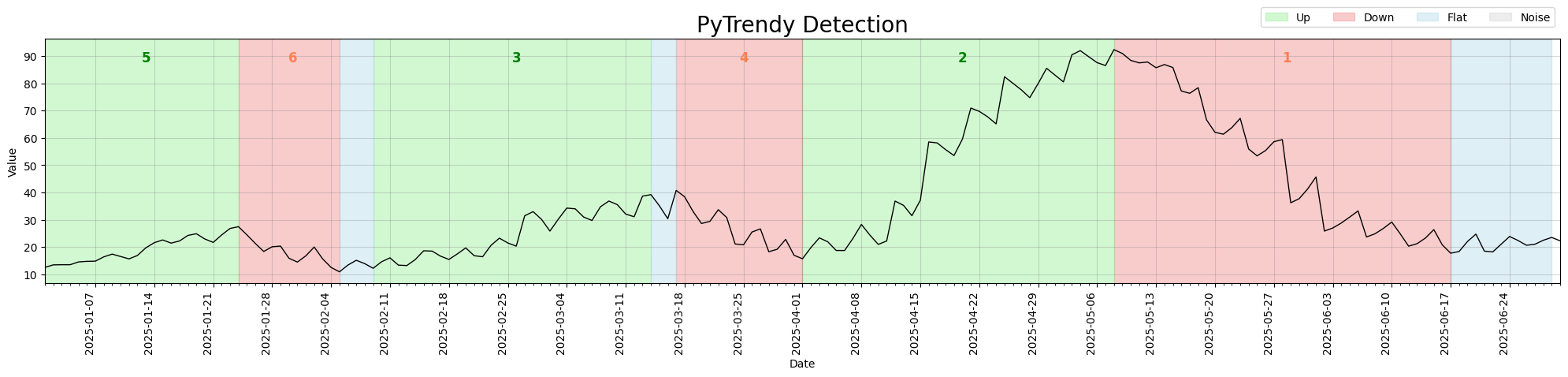
Detected:
- 3 Uptrends.
- 3 Downtrends.
- 3 Flats.
- 0 Noise.

The best detected trend is Down between dates 2025-05-09 - 2025-06-17

Full Results:
-------------------------------------------------------------------------------
            direction       start         end  days  total_change  change_rank trend_class
time_index
1                 Up  2025-01-02  2025-01-24    22     14.013348            5     gradual
2               Down  2025-01-25  2025-02-05    11    -13.564214            6     gradual
3               Flat  2025-02-06  2025-02-09     3     -1.168831            9         NaN
4                 Up  2025-02-10  2025-03-14    32     24.632035            3     gradual
5               Flat  2025-03-15  2025-03-17     2      5.660173            7         NaN
6               Down  2025-03-18  2025-04-01    14    -22.721861            4     gradual
7                 Up  2025-04-02  2025-05-08    36     72.611833            2     gradual
8               Down  2025-05-09  2025-06-17    39    -73.253968            1     gradual
9               Flat  2025-06-18  2025-06-30    12      3.910534            8         NaN
-------------------------------------------------------------------------------
Explore the strongest uptrends:
results.filter_segments(direction='Up', sort_by='change_rank')[:3]
| time_index | direction | start | end | trend_class | change | pct_change | days | total_change | SNR | change_rank |
|---|---|---|---|---|---|---|---|---|---|---|
| 7 | Up | 2025-04-02 | 2025-05-08 | gradual | 72.61 | 367.50% | 36 | 72.61 | 21.70 | 2 |
| 4 | Up | 2025-02-10 | 2025-03-14 | gradual | 24.63 | 169.22% | 32 | 24.63 | 18.87 | 3 |
| 1 | Up | 2025-01-02 | 2025-01-24 | gradual | 14.01 | 104.41% | 22 | 14.01 | 22.21 | 5 |
filter_segments ranks segments by magnitude (change_rank). See the API reference for all filter and sort options.
For the full per-segment metrics table, use results.df.
For more examples on interpreting the results, see Detect Gradual Trends.